# Welcome to Qiskit crash course notes!
## Change qiskit plots' color:
1. find the style definitions inside the package
2. Parse it and caclulate the complementary colors of every color
## Useful links:
* https://serennu.com/colour/rgbtohsl.php
* https://www.easyrgb.com/en/math.php
# Lecture 1: The Atoms of Computation
# Lecture 2: Hello qiskit
# Lab 1
## Notes
- Transpiler `QuantumCircuit.decompose()`
- quantum circuit optimization
## Questions:
1. Why the `str` inside the square brackets in `prob = output1[str(int( input1=='1' and input2=='1' ))]/8192`?
No idea
# Lecture 3: Qubit States and Gates
* https://qiskit.org/textbook/ch-states/representing-qubit-states.html
* https://qiskit.org/textbook/ch-states/single-qubit-gates.html
## Questions
1. Why don't we see the eigenvalues in the Bloch sphere?
2. How to express things on the Bloch sphere using different Bases. I. e. how to express $|\psi\rangle$ as a function of $|+\rangle$ and $|-\rangle$ by looking at the Blochsphere? (This question was triggered by *Quick Exercise 1.* in 3)
# Lecture 4: Multiple Qubit and Entangles States
* https://qiskit.org/textbook/ch-gates/multiple-qubits-entangled-states.html
* https://qiskit.org/textbook/ch-gates/phase-kickback.html
* https://qiskit.org/textbook/ch-gates/more-circuit-identities.html
## General remarks
* Two ways of using the backends:
```python
# Use the unitary simulator to get the whole circuit as a gate
unisim = Aer.get_backend('unitary_simulator')
qc = QuantumCircuit(2)
qc.x(0)
qc.h(1)
display(qc.draw())
display(execute(qc, unisim).result().get_unitary())
unisim = Aer.get_backend('unitary_simulator')
qc = QuantumCircuit(2)
qc.x(0)
qc.h(1)
display(qc.draw())
qobj = assemble(qc)
display(unisim.run(qobj).result().get_unitary())
```
* Qiskit calculates the tensor product backwards w.r.t Qutip, be careful!
* Qiskit counts qubits from the last: |qn...q0> representes the joint state of q0, ..., qn
* **Phase Kickback is important. Practice it!**
## Phase Kickback
### Notes:
1. In a controlled gate, if the control qubit is in a superposition, the eigenvalue of the gate on the target qubit gets "kicked back" to the control qubit as a relative phase.
2. For Z rotations, it does not matter who the control is, the phase of the eigenvalue of the qubit in the z axis gets kicked back to the one that is in a superposition
### Questions
1. How to apply an unitary to a circuit? Can we only use the preshipped gates?
--> 1. search [here](https://learn.qiskit.org/course/ch-gates/basic-circuit-identities)
# Lecture 5: Fun with Matrices
* https://qiskit.org/textbook/ch-gates/proving-universality.html
# Lecture 6: Circuits and Universality
* [same as below?](https://qiskit.org/textbook/ch-gates/proving-universality.html?utm_source=ON24&utm_medium=Social&utm_campaign=Textbook&utm_content=Lecture-6)
* https://qiskit.org/textbook/ch-gates/proving-universality.html
* https://qiskit.org/textbook/ch-gates/oracles.html
## oracle
Boolean oracle: describe by *unitary* evolution

Phase oracle: useful in conjunction with *phase kickback*

# Lecture 7: Superdense Coding and Teleportation
* https://qiskit.org/textbook/ch-algorithms/deutsch-jozsa.html
* https://qiskit.org/textbook/ch-algorithms/bernstein-vazirani.html
* https://qiskit.org/textbook/ch-algorithms/teleportation.html
* https://qiskit.org/textbook/ch-algorithms/superdense-coding.html
## Notes
* DJ: discover in one shot if an oracle is constant or balanced
* 
* BV: discover in one shot the secret string that the oracle bitwise multiplies with the input
* QT: A, B get entangled pair; A entangles and measures her qubit and Psi, destroying Psi; A sends two bits of classical info to B. B uses bits to apply gates to his qubit and recovers Psi.
* SD: A, B get entangled pair; A encodes 2 bits in her qubit and sends it to B; B recovers the 2 bits but looses the qubit.
## Questions
* Understand the Deutsch-Jozsa algorithm. Try to understand the formulas at the beginning and the worked example. Everything else should be understandable after that.
* Same for the Bernstein-Vazirani algo.
* Same for teleportation
* Same for super dense coding
# Lecture 8: Quantum Algorithms 1
* https://qiskit.org/textbook/ch-algorithms/quantum-fourier-transform.html
* https://qiskit.org/textbook/ch-algorithms/quantum-phase-estimation.html
* https://qiskit.org/textbook/ch-algorithms/superdense-coding.html
## Quantum Fourier Transform
### Notes:
1. TODO: Entender las Mates del principio.
2. QFT: |binary, z-basis> to |binary fraction of 2pi rotations on the equatorial plane or x-basis>
3. Algo: 
4. The first two exercises might be interesting. The third one also, but I love recursion...
### Questions:
1. How do we get x inside the tensorized terms of the Fourier transformed qubits when deriving the intuition of rotations and when carrying out the the QFT quantum circuit, but when we do the worked example for 3 qubits we get x0, x1, x2, increasingly for each term?
1. This is taken from Nielsen Chuang p. 217. There the general formula does not look the same as in the Qiskit derivation. It looks the same as in the 3 qubit example.
2. One should prove the equivalence of both notations, as the one including the x in every term is the intuitive one used for the rotation visualizations.
## Quantum Phase Estimation

### Summary:
1. We want to estimate the phase of the eigenvalue of a gate applied to its eigenvector.
2. For this we do:
1. Prepare a counting register of "counting" qubits initialized in a superposition
2. Tensored it with the eigenvector of the gate we want to analyze
3. Apply increasing repetitions of a controlled gate with its eigenstate as target and the "counting" qubits as control qubits, one after the other.
4. Apply inverse Fourier transform
5. Measure the counting qubits, whose encoded value is 2 to the t times the phase of the eigenvalue that we wanted to get.
3. Essentially we are filling the counting qubits with the fourier transform of the phase we want by making use of phase kickback. Then we transform back to bits in the z-basis, which we can measure.
# Lecture 9: Quantum Algorithms 2
* https://qiskit.org/textbook/ch-algorithms/grover.html
* https://qiskit.org/textbook/ch-quantum-hardware/measurement-error-mitigation.html
* https://qiskit.org/textbook/ch-quantum-hardware/density-matrix.html
## Grover
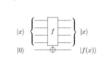
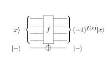
### oracle
### Algo

### Recap real problems:
1. Create a reversible classical circuit that identifies a correct solution
2. Use phase kickback and uncomputation to turn this circuit into an oracle
3. Use Grover's algorithm to solve this oracle
### Questions
1. Where are is the ancilla qubit in the oracle when we implement the circuit? --> If we had our classical funtion $f(x)$, we could construct a reversible oracle using the ancilla qubit. However in this case we just construct the oracles knowing the solution beforehand, to see if the quantum circutits work, as a proof of principle. (see 1. and 2. above)
## Error Mitigation
1. Model *noise* as if the quantum cirquit were perfect and only the measurement part was noisy.
2. Calibrate with state preparation and measurement of all basis vectors
3. assemble noise matrix --> $M_{ij}$ is the probability of mesuring $|i\rangle$ basis vector when preparing $|j\rangle$
4. When doing the actual measurement, multiply the noisy results with the invers of the nois matrix $M^{-1}$


## Density Matrix
### Notes
1. (...) We can then conclude that the reduced density matrix $\rho B$ is a way to describe the statistical outcomes of subsystem $B$, when the measurement outcomes of subsystem $A$ are averaged out. This is in fact what *tracing out* subsystem $A$ means.
# Lecture 10: Quantum Error Correction 1
* https://qiskit.org/textbook/ch-quantum-hardware/error-correction-repetition-code.html
## Notes
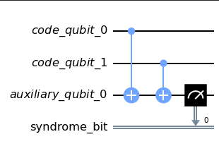
1. Not a good quantum error correction code because it can detect
* bit flips
* phase flips
* but not a the same time
2. I stopped at *graph-theorecic* lookup tables decoding
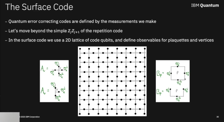
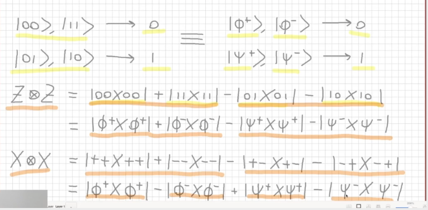
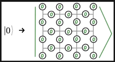
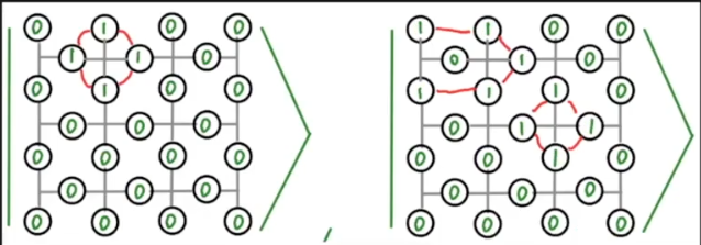
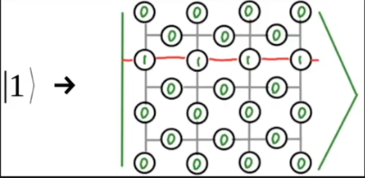
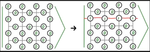
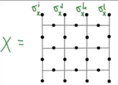
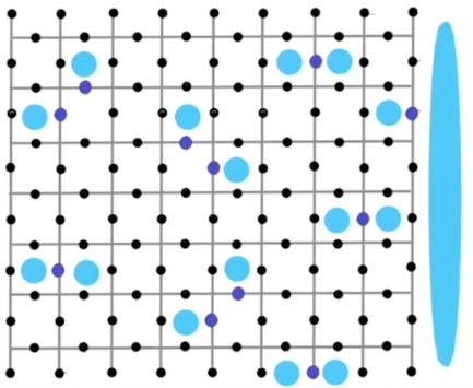
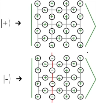
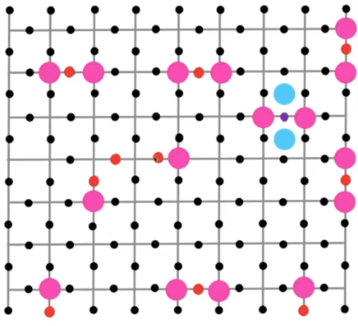
# Lecture 11: Quantum Error Correction 2 (surface codes)
$\varnothing$
## Notes



# Lecture 12: Quantum Machine Learning
slides
* https://github.com/qiskit-community/quantum-fridays/blob/main/Qiskit_friday_QML_intro.pdf
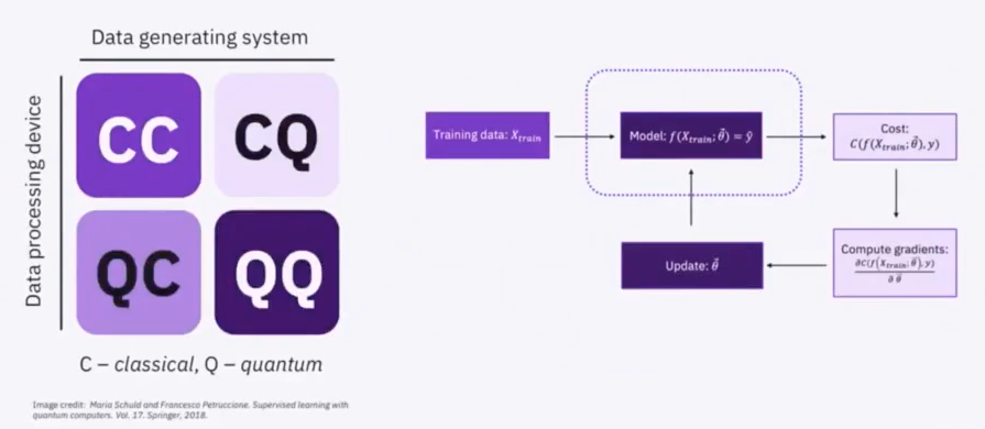
## Recap
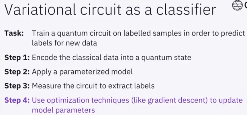
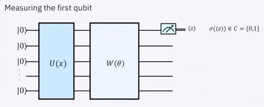
1. Data Encoding
2. Variational Models
3. Optimization
4. Feature Maps
## Shots

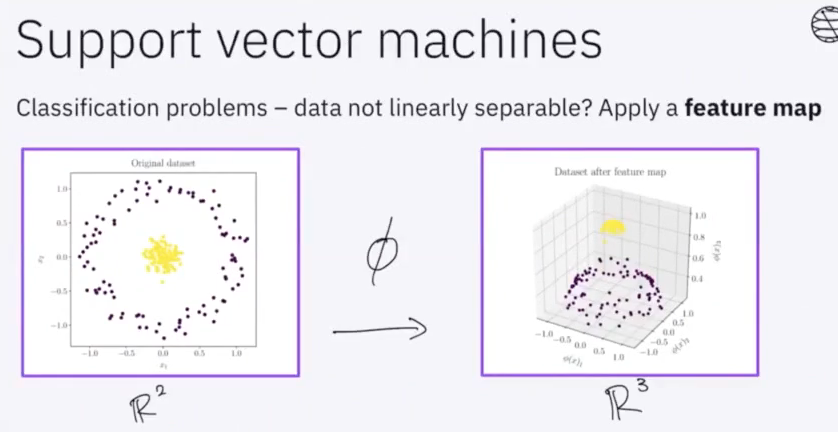
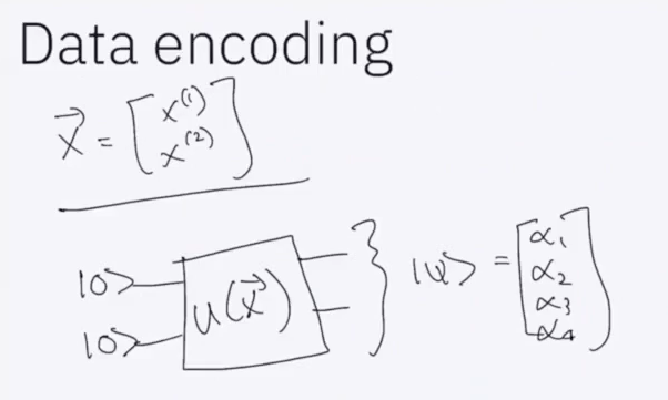
# Lecture 13: Quantum Optimization
notebook
* https://github.com/qiskit-community/quantum-fridays/blob/main/qiskit-optimization.ipynb
## Shots
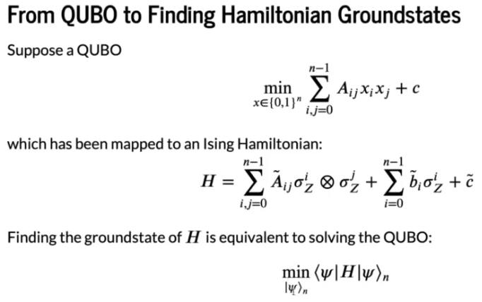
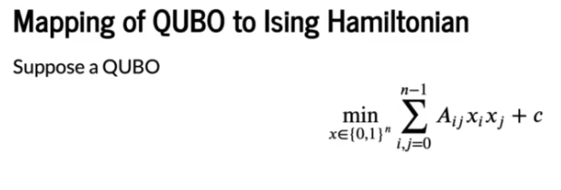
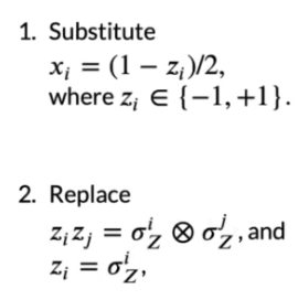
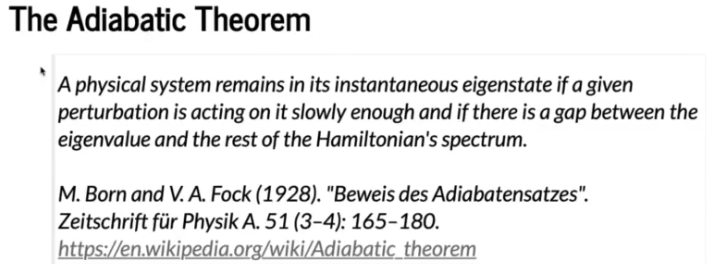
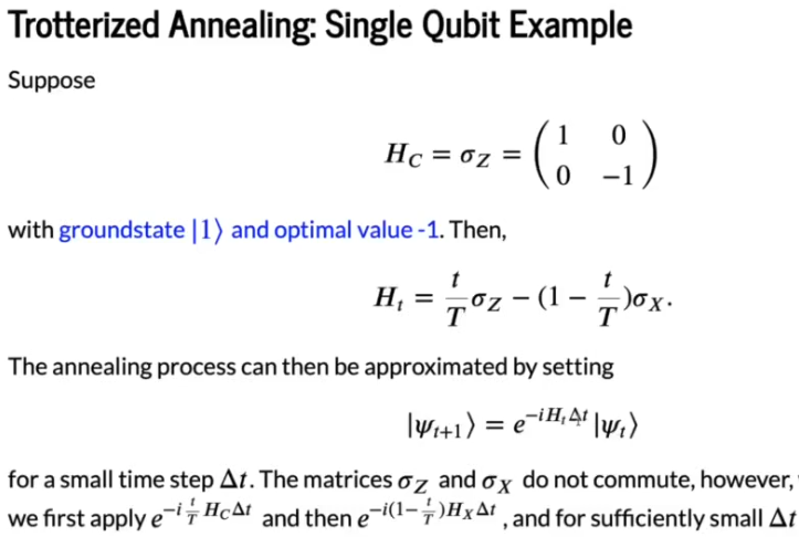
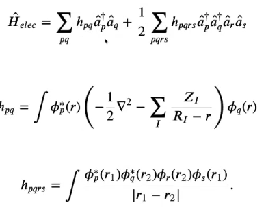
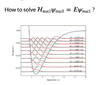
# Lecture 14: Quantum Chemistry
$\varnothing$
## Notes
* Quantum computer need only a linear memory to store it's info
## Shots



# Lecture 15: Quantum Games
$\varnothing$
## Shots


